Certification for Quantum Simulation and Hardware: ZCC-v0.1 and ZHF-v0.1

Everything here is runnable on your own circuit. Try it in the console

Approximate classical simulation has become the practical backbone of near-term quantum research. Matrix product state (MPS) and Pauli propagation methods now reach one hundred qubits and beyond on commodity hardware, and they are the tools most researchers actually use to prototype algorithms, validate hardware, and estimate resources.

Real quantum processors present the same problem from the other direction. A device returns measured counts with no statement of how closely those counts track the ideal answer. Across much of the commercial landscape, both simulated and hardware results are delivered as bare numbers, with no accompanying statement of how far those numbers may sit from the truth.

This omission is consequential, because approximate methods are approximate by construction and physical hardware is noisy by construction, and both characteristic failure modes are silent. The purpose of this article is to make the accuracy statement a first-class output on both sides: to define what can be claimed, to separate evidence from proof, and to specify the two versioned protocols we attach to every job, ZCC-v0.1 for simulated results and ZHF-v0.1 for hardware results.

The failure mode of approximate simulation

A Pauli propagation run with an overly aggressive truncation threshold behaves the same way. Unlike a numerical routine that diverges or a program that crashes, the truncated simulation converges to a confident answer that happens to be incorrect. Any accuracy framework must therefore be designed to detect precisely this quiet, self-consistent kind of error.

Convergence as evidence

The most broadly applicable accuracy check is a convergence study. Every approximate method exposes a resource parameter: the bond dimension for MPS, the coefficient cutoff for Pauli propagation.

Running a circuit at resource level chi and again at 2chi, then measuring the change in the reported observables, yields direct evidence about whether the approximation has saturated. If doubling the resource leaves the result unchanged within tolerance, the additional representational capacity found nothing new.

If the result moves, that movement is itself a quantified warning. This is the same discipline that basis-set convergence and mesh refinement have provided in computational chemistry and numerical analysis for decades.

In the SDK, this is the default behavior for the tensor-network engine. No special flag is required; the convergence record is attached to every result.

import qsim_sdk

client = qsim_sdk.Client(token="...")
job = client.run(circuit, engine="mps.quimb.cpu")

print(job["result"]["error_info"])
# {
#   "method": "MPS (quimb)",
#   "max_bond": 64,
#   "cutoff": 1e-10,
#   "final_max_bond_reached": 2,
#   "convergence_deviation": 0.0,
#   "converged": true,
#   "note": "max |p(chi=64) - p(chi=128)| over top samples"
# }

A convergence check is strong evidence, but it is not a proof. It demonstrates that the answer stopped moving, not that it cannot move. We label it as such and never describe it as a certified bound.

A measured single-run bound

For matrix product states, an accuracy statement is available in a single run, measured rather than extrapolated. When the circuit is built with state renormalization disabled, the squared norm of the final state records exactly how much weight every singular-value decomposition discarded during truncation.

Writing eps for that accumulated discarded weight, eps equals one minus the squared norm of the final state. By the Eckart-Young theorem each individual truncation is optimal, and eps itself is measured exactly rather than estimated. The error on any single outcome probability is then reported as the square root of twice eps.

That figure is tight when the individual truncation errors accumulate incoherently. It is not a worst-case proof: across N sequential truncations the adversarial accumulation is the sum of the square roots of the individual eps values, which can exceed the square root of twice their total by a factor of up to the square root of N over 2.

We report it as a measured bound rather than a guarantee. Pauli propagation is the stricter case. Its bound is an additive triangle inequality over discarded coefficient mass, and needs no such assumption.

We have since tested that assumption rather than resting on it. In deep circuits performing many sequential truncations, the accumulated eps understates the true infidelity by as much as a factor of nine, so the condition the derivation relies on is not always satisfied.

The reported bound is therefore an empirical result: across 334 runs at sizes where the exact answer is computable, 290 of them constructed specifically to falsify it, the figure was never exceeded, coming closest at 49 percent of its value. Those checks need an exact reference and so reach 20 qubits; beyond that size no direct verification is available, and we say so rather than implying the evidence extends further than it does.

We then tried to make the claim stronger, and failed

A second campaign in September 2026 asked a question the first did not. The bound is stated for the error on any single outcome probability, and that is the weakest of several things it might have bounded. Could we honestly claim more? A stronger statement covering the whole distribution at once would be considerably more useful, and the arithmetic looked like it should support one.

So we built six circuit families across 1,543 runs to 24 qubits, three of them designed specifically to break the incoherence assumption rather than to exercise it: one repeating an identical layer so every truncation discards the same direction, one maximising the *number* of tiny truncations, and one using random long-range pairings that an MPS has no locality to exploit. 965 of those runs produced a bound below 1 and were therefore capable of failing. The result:

quantity compared against the bound      exceeded    closest approach
max error on a single outcome           0 / 965          26%
total variation distance               23 / 965         139%
state infidelity                       15 / 965         117%

The claim we publish held, and never came within three quarters of failing. Both stronger claims failed outright. Every violation came from the family built to maximise the number of small truncations, which is precisely the adversarial case the derivation warns about, and the violations grew worse with both circuit size and depth.

We are reporting this because it is the more useful half of the result. The wording on the certificate, the error on any single outcome probability, is not hedging or house style.

It is the strongest statement the evidence supports, and we now know what happens one step beyond it. A protocol that has never been tested to destruction has no idea where its own edges are, and neither do the people relying on it.

One honest caveat, stated because the trend points the wrong way: those violations worsen as circuits grow (1.30x of the bound at 12 qubits, 1.39x at 24), and 24 qubits is where exact verification stops being possible. We cannot see past the point where the evidence runs out, and we do not claim to.

Passing certified=True selects this path, and the reported error_bound is that measured quantity.

job = client.run(circuit, engine="mps.quimb.cpu", certified=True)

print(job["result"]["error_info"])
# {
#   "protocol": "ZCC-v0.1",
#   "method": "MPS (quimb), measured discarded-weight bound",
#   "truncation_weight": 3.2e-09,   # eps = 1 - ||psi||^2
#   "error_bound": 8.0e-05,         # sqrt(2 * eps)
#   "certified": true
# }

Pauli propagation admits the analogous statement. The engine reports the total discarded coefficient mass, which bounds the error on the returned expectation value directly. In both cases the quantity is measured within the run rather than inferred from a second one.

As a concrete, reproducible example, a 192-qubit GHZ circuit measured with an all-Z observable on the pauli.cpu engine returns an expectation value of exactly +1, carrying a certified ZCC-v0.1 error bound of 0 because no Pauli terms were discarded during propagation.

A statevector simulator cannot reach this size, since 192 qubits would demand more memory than exists on Earth, yet the run completed in under a minute for $0.0001, a hundredth of a cent. Its certificate is public and independently verifiable at api.zksf.org/certify/5b8b2c4309d44d41, and the three lines of SDK code that reproduce it are in the documentation.

ZCC-Estimate-v0.2: error mitigation, reported as an estimate

Convergence and the discarded-weight bound both concern classical simulation accuracy. Error mitigation raises a related but distinct question about noisy results: given a measured expectation value, how close is it to the noise-free answer, and how far might the correction still be off?

Zero-noise extrapolation (ZNE) is the standard technique. The circuit is evaluated at several deliberately amplified noise levels and the chosen observable is extrapolated back to the zero-noise limit, which removes much of the coherent bias that gate noise introduces. It runs on the simulator as a cheap preview, and on real hardware, where each noise level is a separate submission, so a three-point extrapolation is three billed runs.

The result carries a ZCC-Estimate-v0.2 statement: the mitigated value together with an uncertainty taken as the larger of the shot-noise uncertainty propagated through the extrapolation and the disagreement between the linear, quadratic, and Richardson extrapolations of the same measured data.

Both quantities are computed without reference to the true answer, so the identical statement applies on hardware, where the true answer is unknown. That makes it an evidence-based statistical estimate rather than the measured ceiling of the certified path. An extrapolated value cannot be bounded with certainty, and the protocol is named and labelled to say so rather than borrowing the authority of a proof it does not have.

What that uncertainty is, measured

Version 0.1 of this protocol reported exactly the arithmetic above and described it as stating how far the mitigation could plausibly be off. That phrasing invites a reader to hear a ceiling, and it is not one. We measured it: 3,312 runs on simulators where the true answer is known, so coverage is checkable rather than assumed.

coverage of the reported interval        simulator 62.4%    hardware 63.7%
what a one-sigma interval implies                    68.3%
multiplier needed to reach 95 percent                2.31x

The arithmetic was never wrong. The shot-noise term is the square root of an intercept variance, which is one standard error, and it behaves like one: roughly two runs in three contain the truth, and one in three does not.

Version 0.2 changes only what is said about the figure. The certificate now states the sigma level in its headline, carries the measured coverage as a field, and says what multiple would be needed for a 95 percent claim.

Two further things fell out of that measurement, and both are reported on the certificate rather than kept in a drawer. The first is counterintuitive: coverage gets worse as you buy more shots, from 76.4 percent at 100 shots down to 47.9 percent at 100,000. More shots shrink the statistical term while leaving the extrapolation's bias untouched, and the bias is the part the interval was missing all along.

The second is more uncomfortable, because it is about whether the technique is worth buying at all. Extrapolating to zero noise amplifies shot noise, so below roughly 10,000 shots on hardware the variance it adds can exceed the bias it removes.

Measured: the mitigated value beat the unmitigated one in 46.9 percent of runs at 1,024 shots and 43.4 percent at 100, against 62.5 percent at 10,000. A job below that threshold now returns an advisory saying so and pointing at the raw value for comparison.

The measurement that found the feature was not running at all

Zero-noise extrapolation amplifies noise by *folding*: replacing the circuit U with U, U-inverse, U, which is mathematically the same operation and three times the gates. That construction is also precisely what an optimising compiler is built to delete.

We checked what the hardware actually executed rather than assuming. IQM returns the compiled program it ran, so the comparison is direct. Submitting folded circuits and letting the provider compile them:

scale   we submitted   the device ran
  1               9               11 gates
  3              27               11 gates
  5              45               11 gates

Every noise level ran the same eleven gates. The compiler had cancelled every folded pair, so all three measurements were of one identical circuit, the extrapolation through three identical points returned the unmitigated value, and the job was billed as three hardware tasks.

The same defect was present on the simulator, where it was circuit-dependent and therefore harder to see: transverse-field Ising and QAOA circuits amplified correctly while a plain rotation-and-CNOT circuit collapsed to a noise spread of one part in 10^15.

The fix is to fold *after* compilation rather than before, in the device's own gate set, and submit the result verbatim so the compiler is not invited to try again. Re-measured on the same device, same circuit:

scale   we submitted   the device ran
  1              14               14 gates
  3              42               42 gates
  5              70               70 gates

We report this for the same reason we report the coverage figures. A mitigation feature that silently does nothing is indistinguishable, from the outside, from one that works. It returns a plausible number with an uncertainty attached. The only way to know is to check what the machine ran, and the only reason we could check is that the provider reports it.

job = client.run(circuit, engine="noisy.cpu", mitigate=True,
                 observable=[[1.0, "ZZ"]])

print(job["result"]["error_info"])
# {
#   "protocol": "ZCC-Estimate-v0.2",
#   "technique": "zero-noise extrapolation",
#   "raw_expectation": 0.81,
#   "mitigated_expectation": 0.82,
#   "error_bound": 5.0e-02,
#   "estimated": true
# }

Most platforms that offer mitigation at all return the mitigated number alone, with no error statement. Reporting the uncertainty, and labelling it an estimate rather than a bound, applies the same discipline to a third case: state what can be claimed, and separate evidence from proof.

Click to enlarge

Close

Reproducible benchmarks

The following runs are drawn from our internal benchmark suite. The CPU figures are from a single consumer laptop (Intel i7-12700H, 32 GB RAM); the 32-qubit statevector is from the GPU tier. The circuits themselves are standard and stated in full below, so an equivalent suite can be assembled with any Qiskit-compatible stack.

Circuit                        Qubits  Depth  Engine          Wall time  Accuracy
GHZ (Clifford)                 5,000   5,000  clifford        0.56 s     exact
QAOA MaxCut ring, p=3          100     304    mps.quimb.cpu   5.9 s      converged (dev 0.0)
Hardware-efficient ansatz      100     9      mps.quimb.cpu   5.6 s      converged (dev 0.0)
Exact reference (ansatz)       26      9      exact.cpu       2.7 s      exact (ground truth)
GHZ exact statevector (GPU)    32      32     exact.gpu       8.2 s      exact (64 GiB state)

The convergence verdicts above are not decorative. Each MPS entry was recomputed at double the bond dimension, and the maximum shift in the leading outcome probabilities was zero to the reported precision. Where an exact reference is tractable, as in the 26-qubit statevector row, the approximate engines reproduce it.

ZHF-v0.1: the hardware analogue

The same infrastructure certifies a different and complementary claim on real hardware. A quantum processor returns its own measured counts, and the relevant statement is device fidelity rather than approximation error, so it carries its own protocol, ZHF-v0.1, rather than being folded into ZCC-v0.1's simulation-accuracy claim.

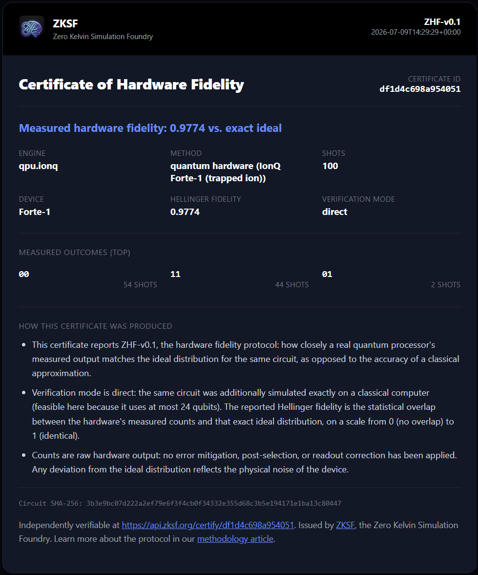
Where the circuit is small enough to also simulate exactly, ZHF-v0.1 reports the measured fidelity between the hardware counts and that exact ideal distribution, computed directly rather than taken from a vendor specification sheet. Two representative runs, submitted through the same API as a simulator job and reported exactly as measured:

Rigetti Cepheus-1-108Q   3-qubit GHZ, 50 shots    000: 23, 111: 22, plus 5 bit-flip errors   45/50 in the GHZ states
IonQ Forte-1             2-qubit Bell, 100 shots   00: 54, 11: 44, 01: 2                        98/100 in the Bell states

These are raw counts with no error mitigation applied. Reported as a live, session-specific fidelity rather than a vendor specification sheet, such measurements are the honest hardware analogue of a simulation error bar. The certificate for the IonQ run above, generated directly from this platform, is shown below.

Where a naive comparison breaks: photonic hardware

Both runs above are gate circuits, where every shot returns a bitstring and the ideal distribution covers all of them. Photonic hardware is not like that, and it forced the protocol to be explicit about something a gate device lets you leave implicit.

On Quandela Belenos, photons are lost in the optics. The device declares a transmittance near 0.05, so most detections register fewer photons than were sent. The exact reference is the lossless distribution and assigns probability zero to every one of those outcomes.

Compared against it directly, a 10,000-shot run scores a Hellinger fidelity of 0.0262, which reads as a device that does not work. The same run bunched 262 of its 271 two-photon detections correctly, which is the interference the experiment was testing.

Both numbers are arithmetically correct and only one answers the question. ZHF-v0.1 therefore reports photonic fidelity conditioned on detecting every photon sent, the standard convention for a lossy optical measurement, and prints the unconditioned figure and the surviving fraction beside it: certificate 063a6fcb82a9464a reports 0.9666 conditioned, 0.0262 unconditioned, over 271 of 10,000 detections.

Stating which subspace a fidelity refers to is not a footnote here. A post-selected number presented as an unconditional one is precisely the overclaim these protocols exist to prevent, and the conditioning is named in the record, in the note, and on the certificate page.

Verifiable certificates, and why verification matters

An error bound printed in a terminal is only as trustworthy as the person who ran the job. Once a number leaves that session and enters a paper, a slide deck, or a client report, its provenance is gone.

A reader has no way to confirm the circuit that was actually run, the method that produced the figure, or whether the number was transcribed correctly. This is not a hypothetical concern. Simulation results are increasingly cited as evidence in hardware comparisons and algorithm papers, and an unverifiable number is, in practice, an assertion rather than a result.

Any completed job can be exported as a certificate that closes this gap. Each certificate is a self-contained record, independent of the account that generated it, that anyone can check without signing in or trusting the author's transcription. A certificate carries:

• The exact circuit, identified by a SHA-256 hash of its source, so the certificate cannot be silently attached to a different computation
• The method and its parameters: which engine ran the job, and, where relevant, the resource budget used (bond dimension, coefficient cutoff, or the classical direct-verification limit for hardware runs)
• The accuracy verdict: a measured error bound, a convergence-based estimate, or a measured hardware fidelity, labeled according to which of these it is, never blurred together
• A public, permanent verification link, backed by a record containing no account, billing, or personal information, so the certificate can be checked independently of ZKSF as a company

The record behind that link is also served as JSON, at /certify/<cert_id>/json, which makes the check programmatic rather than visual.

zcc-verify is an open-source, dependency-free tool that reads it and recomputes the declared bound from the measurement the certificate reports, requiring the two to agree: the square root of twice the discarded weight for a matrix product state, the discarded coefficient mass itself for Pauli propagation, zero for an exact or stabilizer run.

It runs without an account and does not call this service. What it establishes is that a certificate is well formed and internally consistent, which is not the same as establishing that the underlying measurement was honestly made, and it says so rather than implying otherwise.

A reviewer or collaborator can follow that link and see the same figures the author reported, tied to the same circuit, with no additional trust required. That is the entire purpose of a certificate: to move an accuracy claim from something a reader must take on faith to something a reader can check in one click.

The example below is a 24-qubit QAOA MaxCut ring at depth p=3, run on the certified MPS path at a bond dimension of 48. The bond cap binds during this run, so compression genuinely discards weight rather than representing the state exactly: eps is 5.617e-09 and the resulting bound on any single outcome probability is 1.06e-04. It is shown deliberately in preference to a circuit the simulator can hold exactly, where the bound would be near machine precision and would demonstrate nothing.

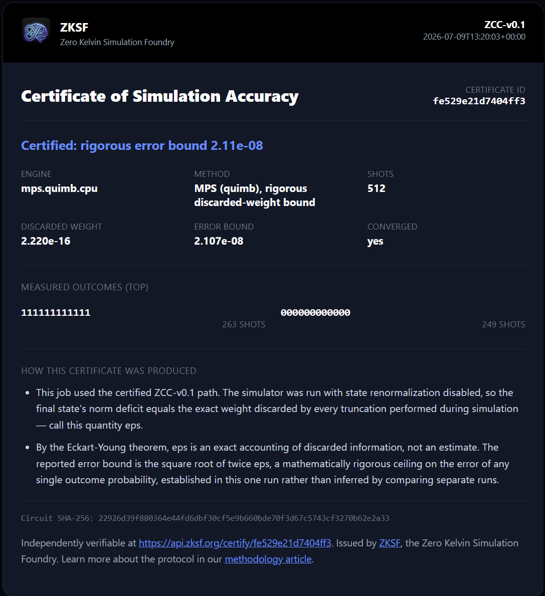
The convergence flag is a separate, stricter test, set far below this bound, so it clears only for runs the simulator represents essentially exactly. The number to cite here is the bound itself: 1.06e-04 on every outcome probability.

Recommendations for practitioners and reviewers

For those reviewing manuscripts, we suggest asking authors what accuracy evidence accompanies any classical simulation baseline, and specifically what a second run at doubled resources would show; for a hardware result, the equivalent question is what fidelity was measured against, and whether that was computed directly or asserted by the vendor. For those procuring simulation or hardware access, the same questions apply to the provider.

A convergence record, a measured truncation bound, and a measured hardware fidelity are all inexpensive to produce and straightforward to verify, and their absence is itself informative. ZCC-v0.1 and ZHF-v0.1 are our attempt to make their presence the default.

The full specification, including the derivations, the validation methodology, and the adversarial falsification search summarized above, is published as a formal, citable paper: Reporting the Accuracy of Approximate Quantum Circuit Simulation: A Machine-Checkable Certificate Format, archived on Zenodo (DOI 10.5281/zenodo.21851381).